... only aspects of the world you haven't modeled yet.
Even the sort of trivially simple setup that's not fit for tutorials (pun not intended) can work as a relevant example. Let's say you're observing the simplest of processes, generating numbers from a gaussian distribution with mean 0 and standard distribution 1, but every now and then, with some probability you don't know but you hope is less than, say, ten percent, the data is corrupted and you just get absolute garbage. (Real projects deal with more complex processes, but seldom with much cleaner measurements.)
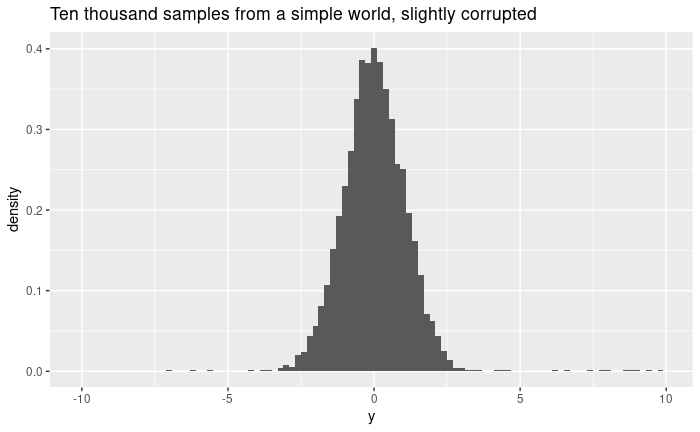
This looks normal-ish enough, and passes with flying colors something like the Shapiro-Wilk's test, so one might as well go and hazard that this "is" a gaussian distribution with mean ~0 and standard deviation... ~1.16. Which is awkward, as we know it's 1.
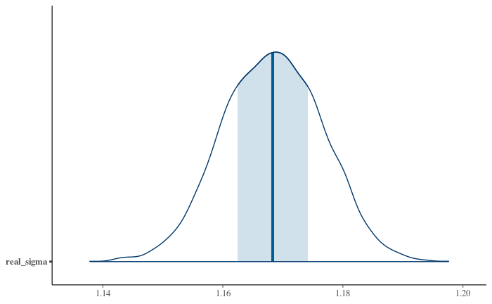
Using a more sophisticated tool to fit the same conceptual model doesn't really help. Here's the distribution of posterior samples for the standard deviation using Stan to fit a gaussian distribution to the data with reasonably scaled priors and good fit diagnostics:
The problem is simply that what's going on isn't "a gaussian plus some errors." It's "mostly a gaussian but sometimes garbage." If you want to model that, then you have to model that. Luckily, it's easy to use something like Stan's log_mix to describe precisely how we think the data generation process goes: with a given probability, you either sample from a gaussian ("the data") or from an uniform distribution ("the error"). Outliers don't come from nowhere, after all: whatever you think it's going on in your data besides the official "good data," whether it's a different population, measurement errors, or anything else, just trying to filter it out or pretend it doesn't exist does you no favors.
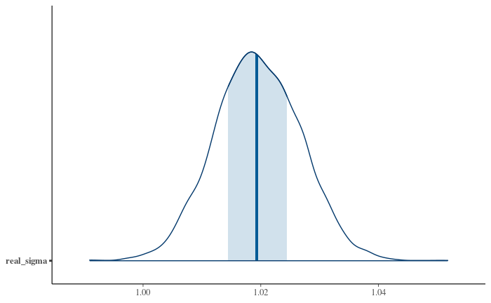
We can fit a model for our data with an explicit outlier-generating process just as well as a simpler one, using data-derived parameters for some of the priors. And just (well, "just") by specifying a more realistic model of your data generation process — one that explicitly says "sometimes the data is pure garbage" — we get a posterior for the standard deviation much better aligned with the true one:
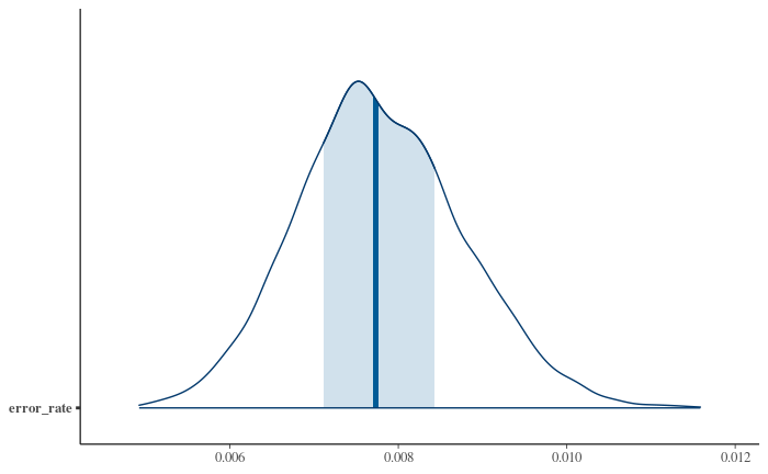
As a bonus, we also get a reasonable estimate of the actual error rate, which I set up as 1% while generating the data; for much lower error rates this discussion is moot, but in a lot of projects I've had to deal with much worse:
The usual way to look at this is that sufficient noise with a large standard deviation will of course bias your estimate of the true standard deviation, such is life, that's why we filter out outliers before fitting models, etc. That's all true, but we can do better.
An slightly more procedural way of expressing the problem is that pretty much all the usual models we fit assume small additive error terms of one sort of another, which is great if those are the sort of errors you have to deal with, but problematic if they aren't. In other words: are you worried about sensors returning 1.12 instead of 1.1
But I think the most general lesson here is that modelling the data generation process — which is what we all do in one way or another, but ideally a deliberate and explicit way — means modeling everything in the path from the real world processes to the numbers in your data table, including your assumptions about error rates and what form those errors take. Understanding the data isn't just about exploring empirical features of a data set before fitting models: it means looking at the business processes, engineering, and often the sociology and psychology of where those numbers are coming from and how they got to your machine. As you can see above, even in unrealistically simple examples a little bit of qualitative knowledge about a data generation process can make a large difference in the quantitative performance of a model.